Multi-Panel Layouts

two_subplots handles the common two-panel case, while n_plotter creates arbitrary grids. Complete signatures and parameter details are available in API Reference.

---

Layout Management

Neither two_subplots nor n_plotter calls tight_layout internally. Call axs.flat[0].get_figure().tight_layout() (or plt.tight_layout()) after plotting if you want tighter spacing.

Both functions return a shaped (n_rows, n_cols) ndarray of Axes. Use axs[row, col] for two-dimensional access or axs.flat[i] for linear indexing. The parent figure is available via axs.flat[0].get_figure().

---

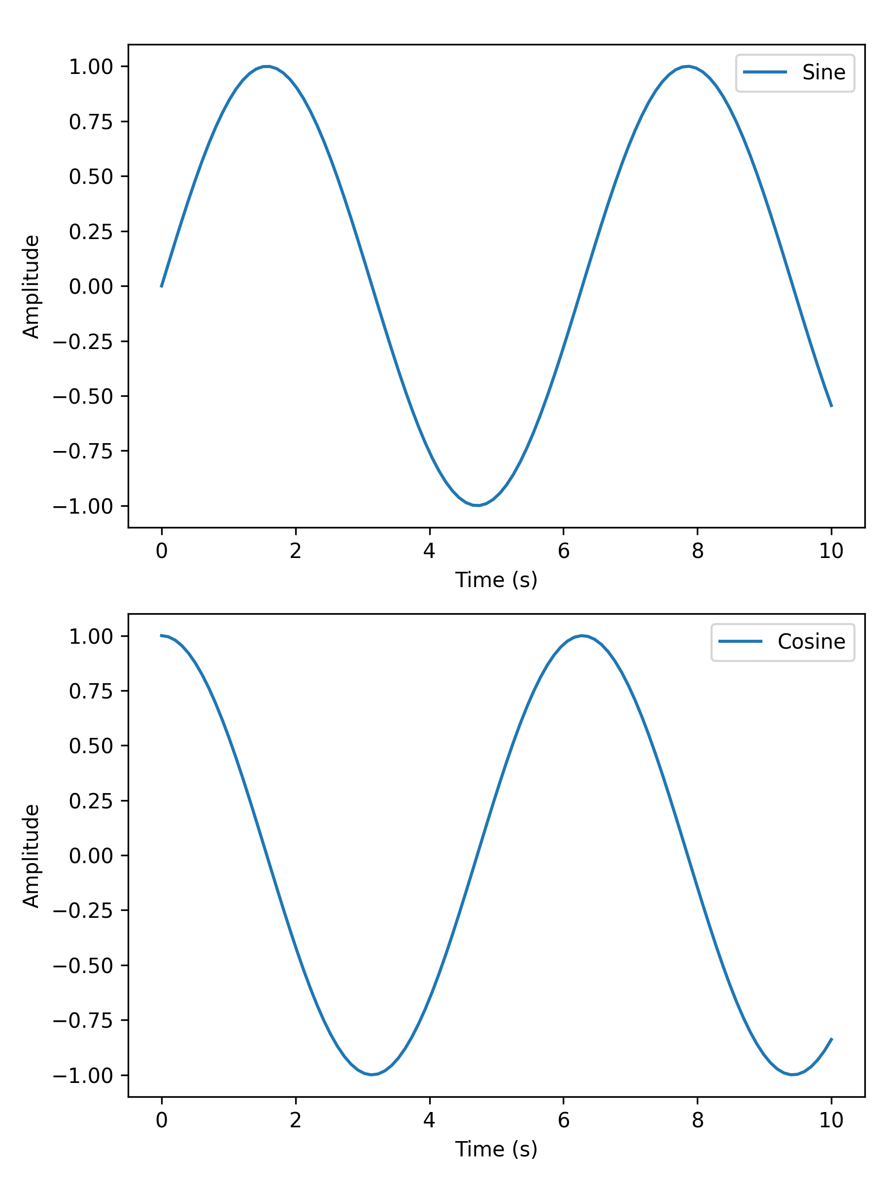
Two Subplots

two_subplots wraps n_plotter for the common two-panel case. Use orientation='h' for side-by-side or 'v' for stacked; subplot_titles labels each panel individually. The return shape is (1, 2) for horizontal layouts and (2, 1) for vertical layouts.

import matplotlib.pyplot as plt
import numpy as np

from plotez import two_subplots

x = np.linspace(0, 10, 100)
y1 = np.sin(x)
y2 = np.cos(x)

two_subplots(
    x_data=[x, x],
    y_data=[y1, y2],
    orientation="v",  # works with both 'v' and 'vertical'
    x_labels=("Time (s)", "Time (s)"),
    y_labels=("Amplitude", "Amplitude"),
    data_labels=("Sine", "Cosine"),
    figure_kwargs={"figsize": (6, 8)},
)

---

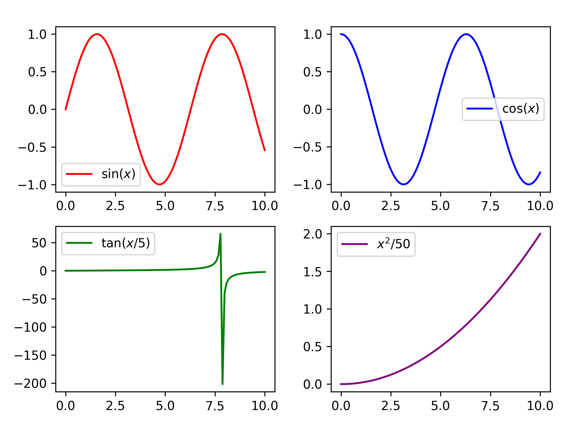
Arbitrary Grids

n_plotter handles arbitrary N x M grids. Config parameters passed as lists apply per subplot, cycling if the list is shorter than the panel count.

import matplotlib.pyplot as plt
import numpy as np

from plotez import n_plotter
from plotez.backend import LinePlotConfig

x_data = [np.linspace(0, 10, 100) for _ in range(4)]
y_data = [np.sin(x_data[0]), np.cos(x_data[1]), np.tan(x_data[2] / 5), x_data[3] ** 2 / 50]

config = LinePlotConfig(color=["red", "blue", "green", "purple"])

n_plotter(
    x_data=x_data,
    y_data=y_data,
    n_rows=2,
    n_cols=2,
    data_labels=[r"$\sin(x)$", r"$\cos(x)$", r"$\tan(x/5)$", r"$x^2$/50"],
    plot_config=config,
)

---

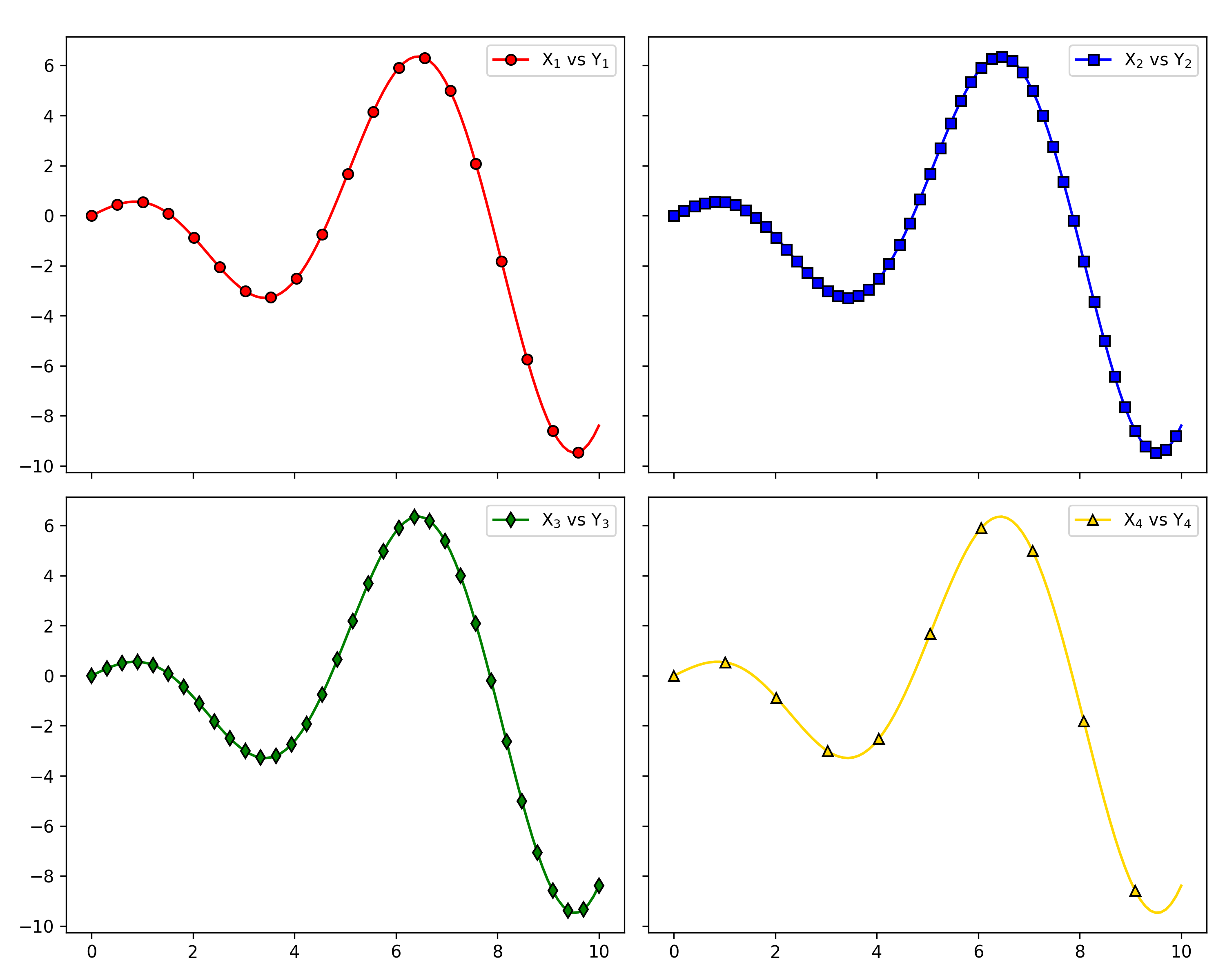
Shared Axes

Pass figure_kwargs={"sharex": True, "sharey": True} to lock axis ranges across all panels; redundant tick labels are hidden automatically.

import matplotlib.pyplot as plt
import numpy as np

from plotez import LinePlotConfig, n_plotter

rng = np.random.default_rng(1234)

x_data = [np.linspace(0, 10, 100) for _ in range(4)]
y_data = [x * np.cos(x) for x in x_data]

fig_kwargs = {"sharex": True, "sharey": True, "figsize": (10, 8)}
line_plot_cfg = LinePlotConfig(
    color=["red", "blue", "green", "gold"],
    markeredgecolor=["k"] * 4,
    marker=["o", "s", "d", "^"],
    _extra={"markevery": [5, 2, 3, 10]},
)

n_plotter(
    x_data=x_data,
    y_data=y_data,
    n_rows=2,
    n_cols=2,
    plot_config=line_plot_cfg,
    figure_kwargs=fig_kwargs,
    data_labels=["X$_1$ vs Y$_1$", "X$_2$ vs Y$_2$", "X$_3$ vs Y$_3$", "X$_4$ vs Y$_4$"],
)